Vector Spaces

Formally, a vector space is a set of objects, called vectors. However, it is important to note that word “vector” in algebra has a much broader sense than just pointy arrows with direction and magnitute. A vector just means an element of a vector space. A suitable candidate for such an element might very well be a whole matrix or even a function.

Thinking in such an abstract way can be extremely practical but one needs to have some boundaries in defining his thoughts in order to make sense and be useful to others. To qualify as a vector space, the set of objects, which I would refer to as \(V\), and the operations which are used on them must adhere to a number of requirements called axioms:

1. Associativity of addition : \(u + (v + w) = (u + v) + w\)
2. Commutativity of addition : \(u + v = v + u\)
3. Identity element of addition : There exists an element \(0 \in V\), called the zero vector, such that \(v + 0 = v\) for all \(v \in V\).
4. Inverse elements of addition : For every \(v \in V\), there exists an element \(−v \in V\), called the additive inverse of \(v\), such that \(v + (−v) = 0\).
5. Compatibility of scalar multiplication with field multiplication: \(a(bv) = (ab)v\)
6. Identity element of scalar multiplication : \(1v = v\)
7. Distributivity of scalar multiplication with respect to vector addition : \(a(u + v) = au + av\)
8. Distributivity of scalar multiplication with respect to field addition : \((a + b)v = av + bv\)

These axioms seem a bit tedious but they have the important task of defining a rigorous frame that if followed correctly is sure to work as expected. Now that everything is defined we can look at some examples. Some of the most important vector spaces are denoted by \(\mathbb{R^n}\). This is also known as the “n-dimensional real space”. Each space of \(\mathbb{R^n}\) consists of \(n\) dimensional real number vectors. For example \(\mathbb{R^5}\) contains all columns vectors with five components and one of these vectors is :

\[v = \begin{pmatrix} 1 \\ 2 \\ 3 \\ 4 \\ 5 \\ \end{pmatrix}\]

Five dimentional space is a bit hard to explore though, since we are living in the three dimentional world and are not used to thinking so abstract. Let’s go to Flatland for a moment and see how everything works in 2D.

If we have two vectors \(v\) and \(w\) in the same vector space \(\mathbb{R^2}\), every linear combination of them in the form \(x = cv + dw\) for some scalars \(c\) and \(d\) should also be in \(\mathbb{R^2}\).

%matplotlib inline 
import numpy as np
import matplotlib.pyplot as plt
import seaborn as sns
sns.set()
#Define Scalars
c = 1.5
d = -1
# Start and end coordinates of the vectors
v = [0,0,1,3]
w = [0,0,2,1]
colors = ['k','silver','silver','orange','k']
x_ = np.array([c*v[2],c*v[2]+d*w[2]])
y_ = np.array([c*v[3],c*v[3]+d*w[3]])
qx = np.array([d*w[2],c*v[2]+d*w[2]])
qy = np.array([d*w[3],c*v[3]+d*w[3]])

plt.figure(figsize=(20,6))
plt.subplot(1,2,1)
plt.plot(x_,y_, color = "silver", dashes = [4,4], zorder = 0)
plt.plot(qx,qy, color = "silver", dashes = [4,4], zorder = 0)
plt.quiver([w[0],c*v[0],d*w[0],c*v[0]+d*w[0],v[0]],
           [w[1],c*v[1],d*w[1],c*v[1]+d*w[1],v[1]],
           [w[2],c*v[2],d*w[2],c*v[2]+d*w[2],v[2]],
           [w[3],c*v[3],d*w[3],c*v[3]+d*w[3],v[3]],
           angles='xy', scale_units='xy', scale=1, color = colors)
plt.xlim(-5, 5)
plt.ylim(-2, 5)
# Draw axes
plt.axvline(x=0, color='#A9A9A9')
plt.axhline(y=0, color='#A9A9A9')
# Draw the name of the vectors
plt.text(0.2, 2, r'$\vec{v}$', size=18)
plt.text(1.25, 0.00, r'$\vec{w}$',  size=18)
plt.text(-1, 2, r'$\vec{x}$',  size=18)

plt.show()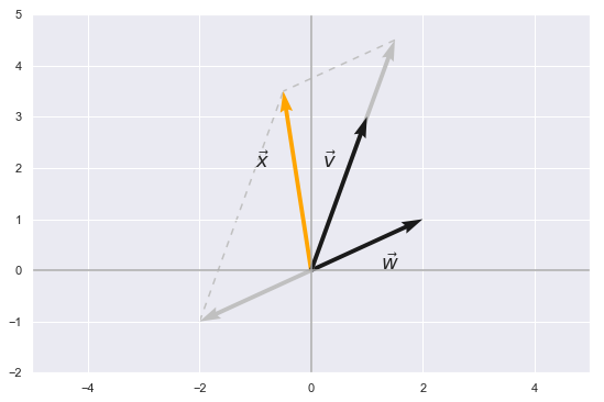

In the above case we scaled \(v\) by 1.5 and \(w\) by -1. The result of their addition unsuprisingly is a vector in \(\mathbb{R^2}\) and doesn’t leave the 2D plane that is drawn. In fact, regardless of the choice of scalars every vector that we come up with will still be in this plane or i.e. the same set \(\mathbb{R^2}\). In mathematics this is also called closure under addition and scalar multiplication.

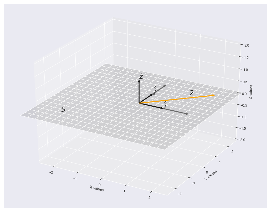
This actually gives rise to the idea of actually thinking about all possible linear combinations as a whole. Specifically, if we have a set of arbitrary vectors \(\{v_1,v_2,...,v_n\} \in V\), then the set of \(c_1v_1 + c_2v_2 + ... + c_nv_n\) for all scalars \(c_1,c_2,...,c_n\) represents something we call the span of the set of vectors. A natural question follows. If we take this span as something on its own can we regard it as another vector space? Intiutively, it makes sense but let’s actually use the eight axioms mentioned earlier. If they apply to the definition of span then we have ourselves a vector space - easy:

\[c_1v_1 + (c_2v_2 + ... + c_nv_n) = (c_1v_1 + c_2v_2 + ...) + c_nv_n\] \[c_1v_1 + c_2v_2 + ... + c_nv_n = c_nv_n + c_{n-1}v_{n-1} + ... + c_1v_1\] \[c_1v_1 + c_2v_2 + ... + c_nv_n + 0 = c_1v_1 + c_2v_2 + ... + c_nv_n\] \[c_1v_1 + c_2v_2 + ... + c_nv_n - c_1v_1 + c_2v_2 + ... + c_nv_n = 0\] \[c_1v_1(c_2v_2 ... c_nv_n) = (c_1v_1c_2v_2 ...)(c_nv_n)\] \[1(c_1v_1 + c_2v_2 + ... + c_nv_n) = c_1v_1 + c_2v_2 + ... + c_nv_n\] \[a(c_1v_1 + c_2v_2 + ... + c_nv_n) = ac_1v_1 + ac_2v_2 + ... + ac_nv_n\] \[(a_1 + a_2 + ... +a_n)(c_1v_1 + c_2v_2 + ... + c_nv_n) =\\ a_1(c_1v_1 + c_2v_2+ ... + c_nv_n) +\\ a_2(c_1v_1 + c_2v_2+ ... + c_nv_n) + ...\\ a_n(c_1v_1 + c_2v_2+ ... + c_nv_n)\]

It seems that the span of vectors is indeed a vector space (no surprise here). However since it is contained within another vector space \(V\), we define it as a subspace. In this case our Formally, any vector space \(V'\) is a subspace of \(V\) if its every element is also an element of \(V\). To solidify all of this let’t plot an example of the span of two vectors \(\hat{i}\) and \(\hat{j}\) with length 1 which would form a subspace \(S\) of \(\mathbb{R^3}\).

from mpl_toolkits.mplot3d import Axes3D
from mpl_toolkits.mplot3d import proj3d
from matplotlib.patches import FancyArrowPatch

class Arrow3D(FancyArrowPatch):
    def __init__(self, xs, ys, zs, *args, **kwargs):
        FancyArrowPatch.__init__(self, (0,0), (0,0), *args, **kwargs)
        self._verts3d = xs, ys, zs

    def draw(self, renderer):
        xs3d, ys3d, zs3d = self._verts3d
        xs, ys, zs = proj3d.proj_transform(xs3d, ys3d, zs3d, renderer.M)
        self.set_positions((xs[0],ys[0]),(xs[1],ys[1]))
        FancyArrowPatch.draw(self, renderer)

fig = plt.figure(figsize=(15,12))
ax = fig.add_subplot(111, projection='3d')

i_2 = Arrow3D([0,2], [0, 0], [0, 0], mutation_scale=10, lw=3, arrowstyle="-|>", color="dimgrey")
ax.add_artist(i_2)
i = Arrow3D([0,1], [0, 0], [0, 0], mutation_scale=10, lw=3, arrowstyle="-|>", color="k")
ax.add_artist(i)
j_2 = Arrow3D([0,0], [0, 2], [0, 0], mutation_scale=10, lw=3, arrowstyle="-|>", color="dimgrey")
ax.add_artist(j_2)
j = Arrow3D([0,0], [0, 1], [0, 0], mutation_scale=10, lw=3, arrowstyle="-|>", color="k")
ax.add_artist(j)
z = Arrow3D([0,0], [0, 0], [0, 1], mutation_scale=10, lw=3, arrowstyle="-|>", color="k")
ax.add_artist(z)
x = Arrow3D([0,2], [0, 2], [0, 0], mutation_scale=10, lw=3, arrowstyle="-|>", color="orange")
ax.add_artist(x)

x, y= np.meshgrid(np.arange(-3, 3, 0.3),
                      np.arange(-3, 3, 0.3))
ax.plot_surface(x, y, np.zeros(x.shape), alpha = 0.2, color = 'silver' )
ax.set_xlabel('X values')
ax.set_ylabel('Y values')
ax.set_zlabel('Z values')
ax.set_xlim3d(-2.5, 2.5)
ax.set_ylim3d(-2.5, 2.5)
ax.set_zlim3d(-2, 2)
ax.text(1, 0, 0, r'$\hat{i}$', color='k',size=22)
ax.text(0, 1, 0, r'$\hat{j}$', color='k',size=22)
ax.text(0, 0, 1, r'$\hat{z}$', color='k',size=22)
ax.text(-2, -2, 0, r'$S$', color='k',size=22)
ax.text(1.2, 1.5, 0, r'$\vec{x}$', color='k',size=20)
plt.show()