Orthogonality and the Gram-Schmidt Algorithm

Orthogonality is a generalization of well known notion of perpendicularity in geometry. The word comes from the Greek ὀρθός (orthos), meaning “upright”, and γωνία (gonia),meaning “angle”. So two vectors in Euclidian space are orthogonal when the angle between them is 90 degrees. If you recall the definition of the dot product

\[a \cdot b = \|a\|\|b\|cos(\theta)\]

you will see that when the angle between the two vectors is \(90^{\circ}\) the \(cos(\theta)\) evaluates to 0 and the whole dot product becomes 0. Which leads to the following simple definition of an orthogonal set: An orthogonal set is a set of vectors, any pair of which have dot product 0.

# Start and end coordinates of the vectors
vectors = [[0,0,1,0],[0,0,1,1],[0,0,0,1],[0,0,-1,1],[0,0,-1,0]]
colors = ['#ffb743','#ff8b43','#ff5943','#ff4e71','#ff4ed0']

plt.figure(figsize=(10,8))
# Draw axes
plt.axvline(x=0, color='#A9A9A9',zorder = 0)
plt.axhline(y=0, color='#A9A9A9',zorder = 0)
for v,c in zip(vectors,colors):
    plt.quiver([v[0]],
           [v[1]],
           [v[2]],
           [v[3]],
           angles='xy', scale_units='xy', scale=1, color = c, zorder = 1)
plt.xlim(-2, 2.5)
plt.ylim(-1, 1.2)
plt.text(0.5, -0.12, r'$\vec{v}$', size=18)
plt.text(0.7, 0.5, r'$\vec{w_1}$', size=18)
plt.text(0.1, 0.75, r'$\vec{w_2}$', size=18)
plt.text(-0.9, 0.5, r'$\vec{w_3}$', size=18)
plt.text(-0.5, -0.12, r'$\vec{w_4}$', size=18)
plt.text(1.5, 1, r'$\vec{v} \cdot \vec{w_1} = $', size=18)
plt.text(2.11, 1, r'$1$', size=18, color = '#ff8b43')
plt.text(1.5, 0.75, r'$\vec{v} \cdot \vec{w_2} = $', size=18)
plt.text(2.11, 0.75, r'$0$', size=18, color = '#ff5943')
plt.text(1.5, 0.5, r'$\vec{v} \cdot \vec{w_3} = $', size=18)
plt.text(2.05, 0.5, r'$-1$', size=18, color = '#ff4e71')
plt.text(1.5, 0.25, r'$\vec{v} \cdot \vec{w_4} = $', size=18)
plt.text(2.05, 0.25, r'$-1$', size=18, color = '#ff4ed0')
plt.show()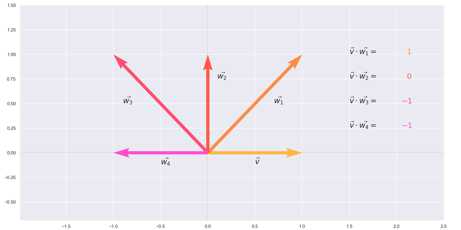

Again, the simplest example of an orthogonal set is the standard basis of \(\mathbb{R^3}\)

\[{(\begin{bmatrix}1\\0\\0 \end{bmatrix}), (\begin{bmatrix}0\\1\\0 \end{bmatrix}), (\begin{bmatrix}0\\0\\1 \end{bmatrix}),}\]

As you may guess this set is also linearly independent and this applies to every orthogonal set of vectors. If all of the vectors in such a set additionally happen to have a norm of 1 then we call the set orthonormal.

Often more than not, orthogonal or orthonormal bases are much easier to work with. Thus, given a basis for a vector space, it is useful to transform it into an orthogonal one. This can be achieved using the Gram-Schmidt algorithm which heavily relies on the concept of projection. So let’s first introduce and explore the projection operator:

\[proj_v(x)= \frac{\langle {v,x} \rangle}{\langle {v,v} \rangle}v\]

The formula can be explained using some visualization.

%matplotlib inline
scalars = np.arange(-7,7,0.35)
v = [0,0,2,2]

plt.figure(figsize=(20,6))
plt.subplot(1,2,1)
plt.quiver([0,0,0,0],
           [0,0,0,0],
           [4,1,2.25,-1.25],
           [4,3.5,2.25,1.25],
           angles='xy', scale_units='xy', scale=1,color = ['#ff4248','#ffb031','#ff7d31','#ffc73a'] ,zorder = 3)
for s in scalars:
    plt.quiver([v[0]],
           [v[1]],
           [s*v[2]],
           [s*v[3]],
           angles='xy', scale_units='xy',color = 'silver', scale=1, zorder = 2)

plt.plot([2.25,1],[2.25,3.5], color = "grey", dashes = [4,4], zorder = 1)
# Draw axes
plt.axvline(x=0, color='#A9A9A9', zorder = 1)
plt.axhline(y=0, color='#A9A9A9', zorder = 1)
plt.axis('equal')
plt.xlim(-5, 7)
plt.ylim(-4, 7)
plt.text(3.35, 2.75, r'$\vec{v}$', size=18)
plt.text(0, 2.25, r'$\vec{x}$', size=18)
plt.text(1.45, 0.75, r'$proj_\vec{v}(\vec{x})$', size=18)
plt.text(-1.9, 0.75, r'$\vec{x} - proj_\vec{v}(\vec{x})$', size=13, rotation = -45)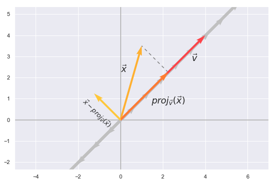

The projection of \(x\) onto \(v\) would be some vector in the span of \(v\) which can be expressed as \(proj_\vec{v}(\vec{x}) =cv\). From the illustration we see that \(x-cv\) happens to be orthogonal to \(v\) therefore \(\langle {x-cv,v} \rangle=0\). If we make use of the distributive property of the inner product it is possible to express \(c\) which is the exact needed scalar to multiply with \(v\) and get the projection.

Now we can use the projection operator to describe the Gram-Schmidt algorithm. Given a basis

\[(v_1,v_2,...,v_n)\]

we make a new set

\[(u_1,u_2,...,u_n)\]

where

\[\begin{align} u_1&=v_1\\ u_2&=v_2-proj_{u_1}(v_2)\\ u_3&=v_3-proj_{u_1}(v_3)-proj_{u_2}(v_3)\\ &\vdots\\ u_n&=v_n-proj_{u_1}(v_n)-proj_{u_2}(v_n) ...- proj_{u_{n-1}}(v_n) \end{align}\]

This produces an orthogonal basis which can be further normalized to become orthonormal by dividing each vector by its magnitute like this:

\[e_1 = \frac{u_1}{\|u_1\|}\\ e_2 = \frac{u_2}{\|u_2\|}\\ \vdots\\ e_n = \frac{u_n}{\|u_n\|}\]

Geometrically, this method proceeds as follows: to compute \(u_i\), it projects \(v_i\) orthogonally onto the subspace \(U\) generated by \(u_1, ..., u_{i−1}\), which is the same as the subspace generated by \(v_1, ..., v_{i−1}\). The vector \(u_i\) is then defined to be the difference between \(v_i\) and this projection, guaranteed to be orthogonal to all of the vectors in the subspace \(U\).What this operation is essentially doing is removing the projection of this \(v_i\) onto U, and leaves only the orthogonal part. In this sense the Gram–Schmidt algorithm is a great way to “rephrase” your basis. When this process is implemented on a computer,however, a problem arises. The vectors \(u_1, ..., u_{i−1}\) often turn out to be not quite orthogonal, due to physical limitations. Round-off errors can accumulate and destroy orthogonality of the resulting vectors. If you execute the algorithm in its pure form (sometimes referred to as “classical Gram–Schmidt”) this loss of orthogonality is particularly bad. Therefore, it is said that the (classical) Gram–Schmidt process is numerically unstable and this calles for a slight modification. Instead of computing a vector \(u_k\) as

\[u_k = v_k - proj_{u_1}(v_k)-proj_{u_2}(v_k)-...-proj_{u_k-1}(v_k)\]

it is better approximated as:

\[\begin{align} u_k^{(1)}&=v_k - proj_{u_1}(v_k)\\ u_k^{(2)}&=u_k^{(1)}-proj_{u_2}u_k^{(1)}\\ &\vdots\\ u_k^{(k-2)}&=u_k^{(k-3)}-proj_{u_{k-2}}u_k^{(k-3)}\\ u_k^{(k-1)}&=u_k^{(k-2)}-proj_{u_{k-1}}u_k^{(k-2)} \end{align}\]

Each step here finds a vector \(u_{k}^{(i)}\) orthogonal to \(u_{k}^{(i-1)}\).

In a sense, the modified Gram-Schmidt (MGS) takes each vector and modifies all of the forthcoming vectors to be orthogonal to it while the original method takes each vector, one at a time, and makes it orthogonal to all the previous vectors. If you think about it the modified Gram–Schmidt process should yield the same result as the original formula if we were to comparing with exact arithmetic.

Here is my Python implementation. As an example I have defined the starting set of vectors to be:

\[(\begin{bmatrix}1\\0\\0 \end{bmatrix}, \begin{bmatrix}1\\1\\0 \end{bmatrix}, \begin{bmatrix}1\\1\\1 \end{bmatrix})\]

import numpy as np

# Set of linearly independent vectors as columns of the matrix V
V = np.array([[ 1, 1, 1],
              [ 0, 1, 1],
              [ 0, 0, 1]])

m = V.shape[0] # Number of rows
n = V.shape[1] # Number of columns
U = np.zeros((m,n)) # Placeholder for the new basis matrix with the same dimensions
for i in range(n):
    U[:,i] = V[:,i]
    for j in range(i):
        U[:,i] = U[:,i] - ((np.dot(U[:,i].T,U[:,j])  / np.dot(U[:,j].T,U[:,j]))*U[:,j])
    U[:,i] = U[:,i]/np.sqrt(np.dot(U[:,i].T,U[:,i])) # Normalize step

print(U)

[[1. 0. 0.]
[0. 1. 0.]
[0. 0. 1.]]

A simple way to check if the columns of the resulting matrix \(U\) are orthogonal is to simply verify that \(U^TU=I\), where \(I\) is the identity matrix.

np.dot(U.T,U)

[[1. 0. 0.]
[0. 1. 0.]
[0. 0. 1.]]