The Inverse and LU Decomposition Agorithms

We usually use a matrix to denote a change, a linear transformation that affects the space we are working with. And almost as if following Newton’s third law which says that every action has an opposing equal reaction, linear transformations in the form of a matrix very often have an inverse which equates to the mechanical reaction. An inverse represents the opposite transformation of the original matrix. Thus, if you first multiply a vector by some matrix say \(A\), and then multiply the resulting vector by the inverse \(A^{-1}\) you would end up with the same vector as if nothing happened to it. The matrix that denotes this lack of change is the identity \(I\). Accordingly, in an equation the statement takes the following form:

\[AA^{-1}=I\]

Another important property of the matrix inverse which follows is that the inverse of the product of two matrices is the product of their individual inverses in the reverse order:

\[(AB)^{-1}=B^{-1}A^{-1}\]

A simple proof can be derived from the forementioned property:

\[(AB)(B^{-1}A^{-1}) = A(BB^{-1})A^{-1} = AA^{-1} = I\]

One immediate application of the inverse is solving systems of linear equations. If we had an system which we would express as \(Ax=b\), then all we would need is to “divide” by it the whole thing so that we get the right vector \(x\). The inverse does just that.

\[x = A^{-1}b\]

But how is this inverse found? The oldest method is well known - Gaussian elimination. This is an algorithm which consists of series of steps over each of the columns in the matrix.

In the context of the algorithm, every diagonal entry of the matrix is referred to as a pivot and the goal is to have all zeroes beneath the pivot positions. This is done sequentially by taking the pivot of each column of the matrix and looking at the entries beneath it. What we are looking for in each of these is a constant. A constant with which to multiply the pivot row. Once multiplied we then substract the pivot row from the selected row.

But instead of explaining the algorithm, let’s view an example. Suppose we have

\[A= \begin{bmatrix} 1 & 1 & 0 & 3\\ 2 & 1 &-1 & 1\\ 3 &-1 &-1 & 2\\ -1& 2 & 3 &-1 \end{bmatrix} \begin{bmatrix} x_1\\ x_2\\ x_3\\ x_4 \end{bmatrix}= \begin{bmatrix} 4 \\ 1 \\ -3\\ 4 \end{bmatrix}\]

The diagonal entries are the pivots and the first one is \(a_{11}=1\). Next we find an appropriate \(c\) to multiply the entry beneath by dividing it by the pivot:

\[\begin{align} c_1 & = 2/1 = 2 \\ c_2 & = 3/1 = 3 \\ c_3 & = -1/1= -1 \\ \end{align}\]

Next, we multiply the pivot row by the corresponding \(c_i\) and substract it from the rows beneath.

\[\begin{align} E_1\\ E_2-2E_1 &\rightarrow E_2\\ E_3-3E_1 &\rightarrow E_3\\ E_4+E_1 &\rightarrow E_4 \end{align} \begin{bmatrix} 1 & 1 & 0 & 3\\ 0 &-1 &-1 & -5\\ 0 &-4 &-1 & -7\\ 0 & 3 & 3 &-2 \end{bmatrix} \begin{bmatrix} x_1\\ x_2\\ x_3\\ x_4 \end{bmatrix}= \begin{bmatrix} 4 \\ -7 \\ -15\\ 8 \end{bmatrix}\]

And we go to the next column, define a vector of \(c_i\)’s and make everything below the pivot zero.

\[\begin{align} E_1\\ E_2\\ E_3-4E_2 &\rightarrow E_3\\ E_4+3E_2 &\rightarrow E_4 \end{align} \begin{bmatrix} 1 & 1 & 0 & 3\\ 0 &-1 &-1 & -5\\ 0 & 0 & 3 & 13\\ 0 & 0 & 0 &-13 \end{bmatrix} \begin{bmatrix} x_1\\ x_2\\ x_3\\ x_4 \end{bmatrix}= \begin{bmatrix} 4 \\ -7 \\ 13\\ -13 \end{bmatrix}\]

The next step would normally aim to make \(a_{43}=0\) accordingly, but this unintentionally is already the case so there is no need in writing it explicitly. A computer program would have to do all of same calculations though. What is more interesting is the fact that the resulting matrix after this routine has only zeroes below the diagonal making it a so-called upper triangular matrix which is often denoted as \(U\). This allows the system of equations to be solved by backward substition, an even simpler algorithm which consists of taking the last row pointing us at \(x_n\), substituting it in the equation above it, solving for \(x_{n-1}\), and then repeat it all over until there are no unknowns left.

Here is a program which does just that:

def backward(U,b):
    '''
    U is an upper triangular square matrix
    b is an nx1 dimensional vector
    '''
    n = len(U)
    x = np.zeros(b.shape)
    for i in range(n-1,-1,-1):
        x[i] = (b[i] - U[i].dot(x.T))/U[i,i]
    return x

A = np.array([[1,1,0,3],
              [0,-1,-1,-5],
              [0,0,3,13],
              [0,0,0,-13]],dtype = float)
b = np.array([4,-7,13,-13])
backward(A,b)

Which returns the following array \(x\):

array([-1.,  2.,  0.,  1.])

And the whole Gaussian Elimination algorithm which solves for \(x\) written with Numpy looks like this:

def gauss_elim(A,b):
    n = len(A)
    U = np.copy(A)
    for i in range(n):#for every column
        for j in range(i+1,n):#for every element under i
            c = c # compute c
            U[j,i:n] = U[j,i:n] - c*U[i,i:n]
            b[j] = b[j] - c*b[i]
    return backward(U,b)

gauss_elim(A,b)

array([-1.,  2.,  0.,  1.])

It’s amazing that this series of simple steps almost magically yield the right result. The first known usage of this algorithm is explained in an ancient chinese book called The Nine Chapters on the Mathematical Art which was written as early as approximately 150 BCE. Much later in Europe the method stemed from the notes of Isaac Newton and Gauss popularized it which resulted in it’s wide known name - Gaussian elimination.

Let’s think for a moment about what the algorithm is actually doing though. It is sequentually applying elementary row transformations on the original matrix. Transformations such as these can also easily be expressed as a matrix. In the first example we did two consecutive iterations over the first two columns which is the same as multiplying the original matrix \(A\) by two elementary matrices. More concisely:

\[\begin{align} \begin{bmatrix} 1 & 0 & 0 & 0\\ -2 & 1 & 0 & 0\\ -3 & 0 & 1 & 0\\ 1 & 0 & 0 & 1 \end{bmatrix} \begin{bmatrix} 1 & 1 & 0 & 3\\ 2 & 1 &-1 & 1\\ 3 &-1 &-1 & 2\\ -1& 2 & 3 &-1 \end{bmatrix}&= \begin{bmatrix} 1 & 1 & 0 & 3\\ 0 &-1 &-1 & -5\\ 0 &-4 &-1 & -7\\ 0 & 3 & 3 &-2 \end{bmatrix}\\ \begin{bmatrix} 1 & 0 & 0 & 0\\ 0 & 1 & 0 & 0\\ 0 &-4& 1 & 0\\ 0 & 3 & 0 & 1 \end{bmatrix} \begin{bmatrix} 1 & 1 & 0 & 3\\ 0 &-1 &-1 & -5\\ 0 &-4 &-1 & -7\\ 0 & 3 & 3 &-2 \end{bmatrix}&= \begin{bmatrix} 1 & 1 & 0 & 3\\ 0 &-1 &-1 & -5\\ 0 & 0 & 3 & 13\\ 0 & 0 & 0 &-13 \end{bmatrix} \end{align}\]

Notice that the matrices that denote the operations are just modified identity matrices with off-diagonal entries corresponding to the different vectors \(c\) in each iteration,that is, \(L_{ij}\) is the multiplier that eliminated \(A_{ij}\). Let’s name them \(E_1\) and \(E_2\). Since matrix multiplication is associative, we can express the following:

\[\begin{align} E_2E_1A=U\\ EA=U \end{align}\]

This resulting matrix E is still lower triangular and in our example is exactly this one:

\[\begin{bmatrix} 1 & 0 & 0 & 0\\ -2 &1 & 0 & 0\\ 5& -4 & 1 & 0\\ -5 & 3 & 0 &1 \end{bmatrix}\]

However, if we rearrange the equation a bit and move \(E\) to the other side as it’s inverse as \(L\),

\[A = LU\]

you’ll find that \(L\) bears a more appealing form. In our example its this one:

\[L = \begin{bmatrix} 1 & 0 & 0 & 0\\ 2 &1 & 0 & 0\\ 3& 4 & 1 & 0\\ -1 & -3 & 0 &1 \end{bmatrix}\]

This is a combination of the first two elementary matrices which were constructed for each of the columns but with an opposite sign. The form is not the only thing that is appealing in the equation above. It tells us that, if you can invert a matrix, then you can decompose it as a product of two matrices, namely a lower triangular \(L\) and upper triangular \(U\).

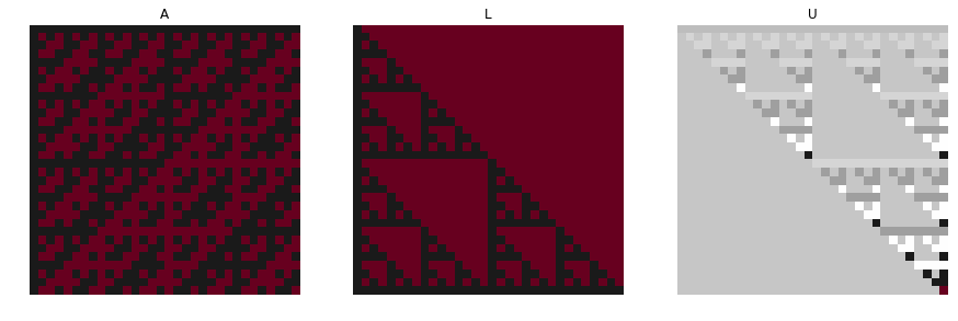
There is an interesting visual example of this decomposition put on Wikipedia. Consider the Haddamard matrix. It’s named after the French mathematician Jacques Hadamard, and it is a square matrix whose entries are either +1 or −1 and whose rows are mutually orthogonal. Here is one of the ways to construct such a matrix expressed as a function:

def Haddamard_M(n):
    '''n must be a power of 2'''
    H = np.array([[1]])
    lg2 = int(np.log2(n))

    # Sylvester's construction
    for i in range(0, lg2):
        H = np.vstack((np.hstack((H, H)), np.hstack((H, -H))))

    return H

W = Haddamard_M(32)

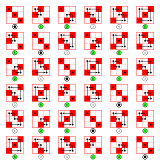
If we try to decompose this particular matrix this is how its corresponding \(L\) and \(U\) matrices would look like:

```python
from scipy.linalg import lu

p,l,u = lu(W)

plt.figure(figsize=(15,10))
plt.subplot(131)
plt.imshow(W,cmap="RdGy")
plt.axis('off')
plt.title("A")
plt.subplot(132)
plt.imshow(l,cmap="RdGy")
plt.axis('off')
plt.title("L")
plt.subplot(133)
plt.imshow(u,cmap="RdGy")
plt.axis('off')
plt.title("U")
```

A natural question arises, if we are able to invert a matrix, why not compute its LU decompostion instead? In reality this is actually what most modern softwares do. The classical Gaussian elimination method more often than not takes too much time when dealing with big matrices, so going straight for the \(LU\) in a clever way is the preferred choice. Once you have the \(LU\) you can then solve for x by rewriting your equation as

\[Ax = LUx = b\]

Then using the notation \(Ux = y\), the equation becomes

\[Ly=b\]

which can be solved for \(y\) with forward substitution, just like backsubstition but in the opposite order.

```python
def forward(L,b):
    '''
    L = an upper triangular nxn matrix,
    b = vector of length n    
    '''
    n = len(L)
    x = np.zeros(b.shape)
    for i in range(n):
        x[i] = (b[i] - L[i].dot(x.T))/L[i,i]
    return x
```

Then,

\[Ux=y\]

will yield the right \(x\) with backsubstitution.

The thing is…, the LU decomposition of a matrix is not unique unless certain constraints are imposed on \(L\) and \(U\). These constraints distinguish one type of decomposition from one another. Here are the three most common ones:

Name	Constraints
Doolittle’s decomposition	\(L_{ii}=1,\:n=1,2,...,n\)
Crout’s decomposition	\(U_{ii}=1,\:n=1,2,...,n\)
Choleski’s decomposition	\(L=U^T\)

Doolittle’s decomposition takes an \(n×n\) matrix \(A\) and assumes that an LU decomposition exists with the constraint that \(L\) has ones across the diagonal. In the case of a 3 by 3 matrix the assumptions leads to the following:

\[L = \begin{bmatrix} 1 & 0 & 0\\ L_{21} &1 & 0\\ L_{31}& L_{32} & 1 \end{bmatrix} U = \begin{bmatrix} U_{11} & U_{12} & U_{13} \\ 0&U_{22} & U_{23} \\ 0& 0 & U_{33} \end{bmatrix} \\ A = \begin{bmatrix} U_{11} & U_{12} & U_{13} \\ U_{11}L_{21}&U_{12}L_{21}+U_{22} &U_{13}L_{21}+U_{23} \\ U_{11}L_{31}&U_{12}L_{31}+U_{22}L_{32} &U_{13}L_{31}+U_{23}L_{32}+U_{33} \end{bmatrix}\]

The algorithm for Doolittle’s decomposition therefore starts by computing one row of \(U\) and one column of \(L\) as follows:

• For the elements of the upper triangular \(U\) we use the following formula:

\[u_{ij} = a_{ij} - \sum_{k=1}^{i-1}u_{kj}l_{ik}\]

The formula for elements of the lower triangular matrix \(L\) is similar, except that we need to divide each term by the corresponding diagonal element of U.

\[l_{ij}= \frac{1}{u_{jj}} (a_{ij}-\sum_{k=1}^{j-1}u_{kj}l_{ik})\]

When implementing it in Python I decided to initiate the two matrices full with zeroes and make use of the dot product instead of raw sums in order to keep the code shorter.

def Doolitle_LU(A):
    U = np.zeros(A.shape)
    L = np.zeros(A.shape)
    np.fill_diagonal(L, 1)
    n = len(A)
    for i in range(n):
        for k in range(i,n):#produces a row of U
            U[i,k] = A[i,k] - L[i].dot(U[:,k])
        for p in range(i+1,n): #produces a column of L
            L[p,i] = (A[p,i] - L[p].dot(U[:,i]))/U[i,i]
    return L,U

Doolitle_LU(A)[1]

array([[  1.,   1.,   0.,   3.],
       [  0.,  -1.,  -1.,  -5.],
       [  0.,   0.,   3.,  13.],
       [  0.,   0.,   0., -13.]])

When doing Crouts decomposition the only difference is that there are ones across the diagonal of \(U\) and the order of computation is swapped.

def Crout_LU(A):
    U = np.zeros(A.shape)
    L = np.zeros(A.shape)
    np.fill_diagonal(U, 1)
    n = len(A)
    for i in range(n):
        for k in range(i,n):#produces a column of L
            U[i,k] = A[i,k] - L[i].dot(U[:,k])
        for p in range(i+1,n):#produces a row of U
            L[p,i] = (A[p,i] - L[p].dot(U[:,i]))/U[i,i]
    return L,U

Crout_LU(A)[1]

array([[  1.,   1.,   0.,   3.],
       [  0.,  -1.,  -1.,  -5.],
       [  0.,   0.,   3.,  13.],
       [  0.,   0.,   0., -13.]])

Again the resulting matrix \(U\) is identical to the upper triangular matrix that results from Doolittle’s LU and Gauss elimination.

The third one is the Choleski’s decomposition \(A = LL^T\). It has two limitations:

• Since \(LL^T\) is always a symmetric matrix, Choleski’s decomposition requires the original \(A\) to be symmetric.

• The decomposition process involves taking square roots of certain combinations of the elements of A. Consequently, to avoid square roots of negative numbers \(A\) must be positive definite.

Sure, these limitations reduce the scope of use of the decomposition but its also its source of strength. Out of the three, Choleski’s decomposition is the most efficient one to compute due to its exploitation of symmetry. Writing it out explicitly we get:

\[A=LL^T\] \[\begin{bmatrix} A_{11} & A_{12} & A_{13} \\ A_{21} & A_{22} & A_{23} \\ A_{31} & A_{32} & A_{33} \end{bmatrix} = \begin{bmatrix} L_{11} & 0 & 0 \\ L_{21} & L_{22} & 0 \\ L_{31} & L_{32} & L_{33} \end{bmatrix} \begin{bmatrix} L_{11} & L_{21} & L_{31} \\ 0 & L_{22} & L_{32} \\ 0 & 0 & L_{33} \end{bmatrix}\\ = \begin{bmatrix} L_{11}^2 & L_{11}L_{21} & L_{11}L_{31} \\ L_{11}L_{21} & L_{21}^2 +L_{22}^2 & L_{21}L_{31}+L_{22}L_{32} \\ L_{11}L_{31} & L_{21}L_{31}+L_{22}L_{32} &L_{31}^2 +L_{32}^2+L_{33}^2 \end{bmatrix}\]

Note that the full matrix is symmetric, as pointed out earlier. We can also observe that a typical element in the lower triangular portion of \(LL^T\) is of the form

\[(LL^T)_{ij}= L_{i1}L_{j1}+...+L_{ij}L_{jj} = \sum_{k=1}^{j}L_{ik}L_{jk} ,\qquad i\geq{j}\]

Taking the term containing \(L_{ij}\) outside the summation, we obtain

\[A_{ij} = \sum_{k=1}^{j-1}L_{ik}L_{jk} + L_{ij}L{jj}\]

If the entry is diagonal, \(i = j\), the solution is

\[L_{jj} = \sqrt{A_{jj}-\sum_{k=1}^{j-1}L_{jk}^2}, \qquad j=2,3,...n\]

For a nondiagonal entry we get

\[L_{ij}=(A_{ij}-\sum_{k=1}^{j-1}L_{ik}L_{jk})/L_{jj},\qquad j=2,3,...n, \quad i=j+1, j+2, ..., n.\]

Again to write this in python I make use of the dot product for simplicity. As an example lets take the symmetric matrix

\[A = \begin{bmatrix} 4 & -2 & 2 \\ -2 & 2 & -4 \\ 2 & -4 & 11 \end{bmatrix}\]

def cholesky(A):
    L = np.zeros(A.shape)
    n = len(A)
    # diagonal
    for i in range(n):
        try:
            L[i,i] = np.sqrt(A[i,i]-np.dot(L[i,0:i],L[i,0:i]))
        except ValueError:
            print("Matrix is not positive definite")
        # under the diagonal
        for x in range(i+1,n):
            L[x,i] = (A[x,i]- np.dot(L[i,0:x],L[x,0:x]))/L[i,i]
    return L

L = cholesky(A)
L.dot(L.T)

array([[ 4., -2.,  2.],
       [-2.,  2., -4.],
       [ 2., -4., 11.]])

In the future I’ll dedicate a post on scenarios when these algorithms fail in practice and ways on how to correct them.