Linear Regression and OLS Matrix Derivative Derivation

Usually Linear Regression is a simple but effective statistical model that finds a wide range of uses, but the main one for it is to model the relationship between a scalar response (or dependent variable) \(y\) and one or more explanatory variables (or independent variables) \(x_1,x_2,..x_n\). In the case of one explanatory variable the model is called Simple Linear Regression. For more than one explanatory variable, the process is called Multiple Linear Regression.

Theoretically speaking, most of the time in machine learning we are aiming at finding the conditional mean of some response variable \(Y\), given the values of the explanatory variables (or predictors) \(X\). In order to do that, we allow to assume that the response variable is an affine function of those values

\[E(Y|X) = f(X)\]

where \(X\) is the dataset in matrix form (also known as the design matrix) with \(m\) rows for the observations and \(n\) dimensions for the feature columns.

Which leads to the formulation of our Linear Regression model in other terms:

\[y = f(X)+ \epsilon\]

where \(x\in \mathbb{R}^n\) are inputs and \(y\in \mathbb{R}\) are the observed function values and \(\epsilon\) is the model error which is inevitable in most practical cases. It is also worth mentioning that this mental framework has become the basis for what is now called Supervised learning, a general way of learning where the answer is already known an we are trying to mimick the process of producing it. This is mainly because of the abstract nature of it components. Both \(f(X)\) and \(\epsilon\) can be define differently depending on the problem at hand.

In the case of Linear regression, \(f(X)\) takes a linear form. And more specificly, it takes the input variables and defines the output as a linear combination of them.

\[\begin{align} y & = f(X) + \epsilon\\ & = 1\theta_0+x_{i1}\theta_1+...+x_{ij}\theta_m+\epsilon,\quad\quad \text{ $i = 1,2,...,m$}\\ & =X\theta + \epsilon \end{align}\]

where the response variable is

\[y = \begin{bmatrix} y_1\\ y_2\\ \vdots\\ y_m \end{bmatrix}\]

, the dataset is the matrix

\[X = \begin{bmatrix} x_1^T \\ x_2^T\\ \vdots \\x_m^T \end{bmatrix} = \begin{bmatrix} 1&x_{11}&\cdots & x_{1n} \\ 1&x_{21}&\cdots & x_{2n}\\ \vdots&\vdots&\ddots&\vdots\\ 1&x_{m1}&\cdots & x_{mn} \end{bmatrix}\]

,the weight parameter vector is \(\theta = \begin{bmatrix} \theta_0 \\ \theta_1 \\ \vdots \\\theta_m \end{bmatrix}\)

and the error vector is \(\epsilon = \begin{bmatrix}\epsilon_1 \\\epsilon_2 \\ \vdots\\\epsilon_m\end{bmatrix}\).

Now lets look into the error part. It too can be define differently, but the most common way when dealing with scalars as output is to take the quadratic loss or Sum of Squared errors. This method of modelling in literature is also known as Ordinary Least Squares or OLS for short:

\[\begin{align} \mathcal{L}(\theta) & = \sum_{i=1}^n (y_i - x_i^T\theta)^2 \\ & = (y - X\theta)^T(y - X\theta) = (y^T-\theta^TX^T)(y-X\theta) \end{align}\]

Our goal is to minimize this function so that our \(f(X)\) is close as possible to \(y\). Since the loss function depends on the parameters \(\theta\), we need to find the best fitting vector, or in other words, to solve for it. One of the approaches here comes from calculus. We can find the derivative of the loss function with respect to the parameter vector, set it to zero and solve, since it is a ordinary quadratic function the only extremum in it should be it’s minimum.

First we can expand the brackets:

\[\begin{align} \frac{d\mathcal{L}}{d \theta} & = \frac{d}{d\theta}(y^Ty - \theta^TX^Ty - y^TX\theta +\theta^TX^T X\theta) = 0 \end{align}\]

\(y^Ty\) doesn’t invole \(\theta\) so it’s dropped. The second term \(\theta^TX^Ty\) can be rewritten as \(\theta^T\tilde{y}\) where \(\tilde{y} = X^Ty\). Since \(\tilde{y}\) and \(\theta\) are in the same dimension \(1{\times}m\) the output will be a scalar \(s\).

\[s = \theta_1\tilde{y}_1 + \theta_2\tilde{y}_2 + ... + \theta_n\tilde{y}_n\]

the derivative vector of which is \(\begin{bmatrix} \tilde{y}_1 \\ \\\tilde{y}_2 \\ \vdots \\\tilde{y}_n \end{bmatrix}\).

Next term \(y^TX\theta\) is actually \((\theta^TX^Ty)^T\) and will have the exact same derivative vector \(\tilde{y}\). And the last one \(\theta^TX^T X\theta\) we rewrite as \(\theta^T\tilde{X}\theta\) where \(\tilde{X} = X^T X\), the symmetric covariance matrix. The result will be a scalar \(s = \sum_{j=1}^n\sum_{i=1}^n \tilde{X}_{ij} \theta_i \theta_j\) . Differentiating with respect to the \(k\)-th element of \(\theta\) we have

\[\sum_{j=1}^n \tilde{X}_{kj}\theta_j + \sum_{i=1}^n \tilde{X}_{ik}\theta_i\]

which in vector form is actually \(\theta^T \tilde{X}^T +\theta^T \tilde{X} = \theta^T(\tilde{X}^T+\tilde{X})\)

since \(\tilde{X}\) is symmetric, however, we can write it as \(2\theta^T \tilde{X}^T\) and from the transpose property we get \(2\tilde{X}\theta\).

Finally we can express

\[\begin{align} -\tilde{y}- \tilde{y} + 2\tilde{X}\theta &=\\ -X^Ty- X^Ty + 2X^TX\theta &= \\ 2X^TX\theta-2X^Ty \end{align}\]

Setting it to zero gives

\[\begin{align} 2X^TX\theta-2X^Ty &= 0 \\ 2X^TX\theta&=2X^Ty\\ X^TX\theta&=X^Ty\\ (X^TX)^{-1} X^TX\theta &= (X^TX)^{-1} X^Ty\\ \theta &= (X^TX)^{-1} X^Ty \end{align}\]

The \(X^TX\theta=X^Ty\) line from above is also known as the normal equation and is sure to minimize the sum of squared differences between the lft and right sides. And so it leads us to the best linear estimate we can make:

\[\hat{y}=X\theta=X(X^TX)^{-1}X^Ty\]

Now lets actually do some experiments and see how it works visually.

```python
import numpy as np
import matplotlib.pyplot as plt
from mpl_toolkits.mplot3d import Axes3D
import seaborn as sns
sns.set()
%matplotlib inline

num_samples = 100

# The mean values of the three dimensions .
mu = np.array([5, 11, 12])

# The desired covariance matrix.
cov = np.array([
        [1.00, 0.85, 0.95],
        [0.85, 1.00, 0.90],
        [0.95, 0.90, 1.00]
    ])

# Generate the random samples.
df = np.random.multivariate_normal(mu, cov, size=num_samples)

# Plot various projections of the samples.
fig = plt.figure(figsize=(15, 13))

# Fourth subplot
ax4 = fig.add_subplot(1, 1, 1, projection= "3d")
ax4.scatter(df[:,0], df[:,1], df[:,2],s = 60)
ax4.set_xlabel(r'$X_{1}$')
ax4.set_ylabel(r'$X_{2}$')
ax4.set_zlabel(r'$y$')

plt.show()
```

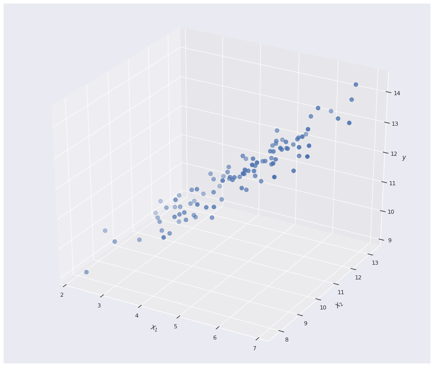
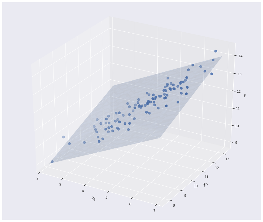
Since we are in the mutivariate setting, the Linear regression model actually forms a 2D plane in \(\mathbb{R^3}\)

```python
# regular grid covering the domain of the data
y = df[:,2]
X = np.delete(df, 2, 1)
# create vector of ones...
I = np.ones(shape=y.shape)[..., None]

#...and add to feature matrix
X = np.concatenate((I, X), 1)
# calculate coefficients using closed-form solution
coeffs = np.linalg.inv(X.transpose().dot(X)).dot(X.transpose()).dot(y)
yhat = X.dot(coeffs)
X = X[:,1:]
mn = np.min(X, axis=0)
mx = np.max(X, axis=0)
X,Y = np.meshgrid(np.linspace(mn[0], mx[0], 100),np.linspace(mn[1], mx[1],100))
# evaluate it on grid
Z = coeffs[1]*X + coeffs[2]*Y + coeffs[0]
fig = plt.figure(figsize=(15,13))
ax = fig.gca(projection='3d')
# Plot the surface.
ax.scatter(df[:,0], df[:,1], df[:,2], s=60)
ax.plot_surface(X, Y, Z,alpha=0.2, linewidth=0, antialiased= True)
plt.xlabel(r'$X_{1}$')
plt.ylabel(r'$X_{2}$')
ax.set_zlabel(r'$y$')
plt.show()
```

In future post I will discuss gometric interpretations of this approach in the language of Linear Algebra and also an alternative method for optimizing the loss function, widely known as Gradient Descent.