Linear Independence, Basis and Dimension

Consider a sample linear combination of two vectors : \(\hat{i} = \begin{bmatrix}1\\0 \end{bmatrix}\) and \(\hat{j} = \begin{bmatrix}0\\1 \end{bmatrix}\) and their \(span(\hat{i},\hat{j}) = \mathbb{R^2}\) which formed a plane.

Let’s see another example however. The set of vectors

\[(\begin{bmatrix}1\\1 \end{bmatrix}, \begin{bmatrix}2\\2 \end{bmatrix}, \begin{bmatrix}4\\4 \end{bmatrix})\]

You can immediately see that they are multiples of each other and if we plot them we can argue that their span is a just line passing through the origin (think about what happens when you scale by a negative number).

#Define Scalars
c = 1.5
d = -1
# Start and end coordinates of the vectors
v = [0,0,1,1]
m = [0,0,2,2]
w = [0,0,4,4]
colors = ['silver','dimgrey','k']

plt.figure(figsize=(20,6))
plt.subplot(1,2,1)
plt.quiver([4*v[0],m[0],v[0]],
           [4*v[1],m[1],v[1]],
           [4*v[2],m[2],v[2]],
           [4*v[3],m[3],v[3]],
           angles='xy', scale_units='xy', scale=1, color = colors)
plt.xlim(-2, 4)
plt.ylim(-2, 6)
# Draw axes
plt.axvline(x=0, color='#A9A9A9')
plt.axhline(y=0, color='#A9A9A9')
plt.scatter(4,7,marker='x',s=50)
# Draw the name of the vectors
#plt.text(0.2, 2, r'$\vec{v}$', size=18)
#plt.text(1.25, 0.00, r'$\vec{w}$',  size=18)
#plt.text(-1, 2, r'$\vec{x}$',  size=18)

plt.show()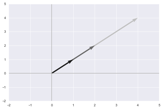

In this example, three vectors formed a mere line, while the two vectors from the first example managed to form a whole plane which is substantionally more ‘spacial’. It would seem that some of the three vectors were ‘redundant’ in a sense that they weren’t adding additional space to the overall span. Mathematically speaking this is known as linear dependence and is defined as follows:

A set of vectors \(\{v_1,v_2,...,v_n\}\) is linearly dependent if there exist constant \(c_1,c_2,...,c_n\) not all 0 such that

\[c_1v_1+c_2v_2+...+c_nv_n=0\]

Otherwise they are linearly independent.

In the example above the constants that prove the linear dependency between the vectors would be \(2,1\) and \(-2\).

\[2\begin{bmatrix}1\\1 \end{bmatrix} + 1\begin{bmatrix}2\\2 \end{bmatrix} + -1\begin{bmatrix}4\\4 \end{bmatrix} = 0\]

Linear independece( or dependence) also provides and interesting look at system of equations. Consider this one:

\[\begin{align} x + 2y = 3 \\ 2x + 6y = 4 \end{align}\]

If you solve it you will get the unique solution of \([x,y] = [5,-1]\) But now consider the system

\[\begin{align} x + 2y = 3 \\ 2x + 4y = 6 \end{align}\]

After a glance at this one, you will most probably conclude that it has an infinite amount of solutions. What you can also notice is that the row vectors \(\begin{bmatrix}1\\2\\3 \end{bmatrix}, \begin{bmatrix}2\\4\\6 \end{bmatrix}\) are actually linearly dependent also.

We can compare the two systems geometrically to get an even better understanding. Let’s first plot the “row picture” of the systems by rearranging and expressing \(y\) in each of the equations and letting \(x\) range.

plt.figure(figsize=(18,6))
plt.subplot(1,2,1)
plt.title("Unique Solution")
plt.xlim(-10, 10)
plt.ylim(-5, 5)
plt.axvline(x=0, color='#A9A9A9')
plt.axhline(y=0, color='#A9A9A9')
x = np.linspace(-10,10)
y = (3-x)/2
plt.plot(x,y, color = '#ff3f35' )
y_1 = (4-2*x)/6
plt.plot(x,y_1, color = '#ff7235')
plt.scatter(5,-1, c = 'brown')

plt.subplot(1,2,2)
plt.title("Infinite Solutions")
plt.xlim(-10, 10)
plt.ylim(-5, 5)
plt.axvline(x=0, color='#A9A9A9')
plt.axhline(y=0, color='#A9A9A9')
x = np.linspace(-10,10)
y = (3-x)/2
plt.plot(x,y)
y_1 = (6-2*x)/4
plt.plot(x,y_1,c = '#ff3589')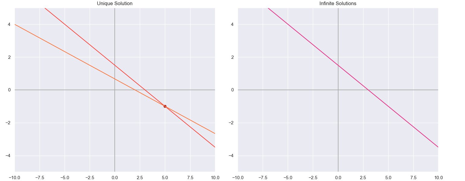

You can clearly see that the unique solution of the first system lies exactly where the two lines intersect in the 2D plane. The second system on the otherhand has infinitely many solutions since the two lines lie ontop of eachother.

We can also get a complimentary “column picture” using the column vectors. In the first system for example they look like this: \(\begin{bmatrix}1\\2 \end{bmatrix}\),\(\begin{bmatrix}2\\6 \end{bmatrix}\) and \(\begin{bmatrix}3\\4\end{bmatrix}\).

#Define Scalars
c = 1.5
d = -1
# Start and end coordinates of the vectors
v = [0,0,1,2]
w = [0,0,2,6]
x = [0,0,3,4]

colors = ['orange','silver','silver','k', 'k']

plt.figure(figsize=(20,6))
plt.subplot(1,2,1)
x_ = np.array([-1*w[2],x[2]])
y_ = np.array([-1*w[3],x[3]])
qx = np.array([5*v[2],x[2]])
qy = np.array([5*v[3],x[3]])
plt.plot(x_,y_, color = "silver", dashes = [4,4], zorder = 0)
plt.plot(qx,qy, color = "silver", dashes = [4,4], zorder = 0)
plt.quiver([x[0],5*v[0],-1*w[0],w[0],v[0]],
           [x[1],5*v[1],-1*w[1],w[1],v[1]],
           [x[2],5*v[2],-1*w[2],w[2],v[2]],
           [x[3],5*v[3],-1*w[3],w[3],v[3]],
           angles='xy', scale_units='xy', scale=1, color = colors, zorder = 1)
plt.xlim(-6, 6)
plt.ylim(-8, 12)
# Draw axes
plt.axvline(x=0, color='#A9A9A9')
plt.axhline(y=0, color='#A9A9A9')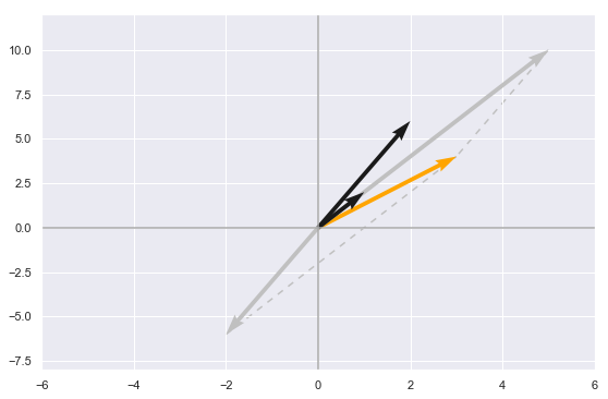

Here by looking at the column vectors we can see that the solution lies in the exact scalar values that multiplied with the first two black vectors will equal the third orange one.

Comparing this to the “column picture” of the second equation we can see that the linear dependence of the column vectors leads to infinite solutions.

#Define Scalars
c = 1.5
d = -1
# Start and end coordinates of the vectors
v = [0,0,1,2]
w = [0,0,2,4]
x = [0,0,3,6]

colors = ['orange','k','k']

plt.figure(figsize=(20,6))
plt.subplot(1,2,1)
x_ = np.array([-1*w[2],x[2]])
y_ = np.array([-1*w[3],x[3]])
qx = np.array([5*v[2],x[2]])
qy = np.array([5*v[3],x[3]])

plt.plot(x_,y_, color = "silver", dashes = [4,4], zorder = 0)
plt.plot(qx,qy, color = "silver", dashes = [4,4], zorder = 0)
plt.quiver([x[0],w[0],v[0]],
           [x[1],w[1],v[1]],
           [x[2],w[2],v[2]],
           [x[3],w[3],v[3]],
           angles='xy', scale_units='xy', scale=1, color = colors, zorder = 2)
plt.xlim(-4, 4)
plt.ylim(-4, 8)
# Draw axes
plt.axvline(x=0, color='#A9A9A9')
plt.axhline(y=0, color='#A9A9A9')
plt.plot(np.arange(-10,10,0.01),np.arange(-10,10,0.01)*2, color='#ff3589', zorder = 1)

#plt.scatter(5,-1, c = 'brown')
# Draw the name of the vectors
#plt.text(0.2, 2, r'$\vec{v}$', size=18)
#plt.text(1.25, 0.00, r'$\vec{w}$',  size=18)
#plt.text(-1, 2, r'$x$',  size=18)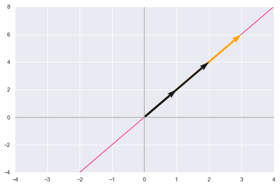

The pictures provide some visual understanding about infinite and unique solutions but you would agree that it is also important to consider the case when no solutions are available. Can we determine generally if a system \(Ax= b\) is solvable? As I mentioned earlier when we seek the solution we are actually seeking the scalars that strech the column vectors just so that when they are added together we get \(b\). Or in other words if \(b\) is a member of the span of the column vectors, the solution can be expressed as a linear combination of the column vectors.

Thinking about spanning space is very awesome but we need to have some orientation in order not to get lost. Mathematicians like to put a marker in the space and orient themselves by it. They call it a basis. But in order to understand what a basis in the context of linear algebra means I think it is best to tackle the formal definition first:

A set of elements (vectors) in a vector space \(V\) is called a basis, or a set of basis vectors, if the vectors are linearly independent and every vector in the vector space is a linear combination of this set. In more general terms, a basis is a linearly independent minimal spanning set of \(V\).

What this means is that if we have a basis set for a vector space \(V\), every element of \(V\) can be expressed uniquely as a linear combination of these basis vectors, whose coefficients are what we are the unit we are measuring with. The simplest example of a basis set is the one which everyone is already using to express things in \(\mathbb{R^3}\) geometrically:

\[{(\begin{bmatrix}1\\0\\0 \end{bmatrix}), (\begin{bmatrix}0\\1\\0 \end{bmatrix}), (\begin{bmatrix}0\\0\\1 \end{bmatrix}),}\]

If we arange the vectors into columns of a matrix we will get the identity operator \(I\). But a vector space can have several distinct sets of basis vectors and that is that is perfectly fine. For example the following set also fits the definition:

\[{(\begin{bmatrix}1\\0\\0 \end{bmatrix}), (\begin{bmatrix}0\\1\\0 \end{bmatrix}), (\begin{bmatrix}0\\1\\1 \end{bmatrix}),}\]

Since we are thinking abstractly we can even define a vector space of third degree polynomials and their basis matrix as follows:

\[\begin{bmatrix} x^3\\x^2\\x\\1 \end{bmatrix}\]

Using functions as a basis is actually pretty useful in machine learning and it is commonly employed as a feaure engineering method. The polynomial expantion in particular allows for approximating non-linear functions with a linear model.

Now let’s move to a related concept: the dimension of a vector space, which is defined as the size of the basis and is denoted as \(dim(V)\). Intuitively we’ve already “seen” that the dimension of \(\mathbb{R^n}\) is \(n\) . Also, if a vector space \(V\) is spanned by a finite set of vectors, then \(V\) is set to be finite-dimensional.

Most of the time the dimension of a subspace is less than the dimension of the original space, which makes dimension a useful tool for thinking about the “size” of a vector space. In fact, more is true: given a basis \(B'\) for a subspace \(V'\) of \(V\), we can extend the basis by adding more vectors to form a basis \(B\) of \(V\).

This becomes important when analyzing bases of subspaces, because we can pick a basis for the subspace, and then pick a basis for the larger space that is guaranteed to be a superset of the original basis.