Norms and Inner Products

If you were to describe a vector you most probably would use its basis to orient it in space and then describe its length and direction. I want to focus on the former property first though - vector length. The concept of length in our three-dimensional physical space is pretty simple but when we are thinking abstractly this can be somewhat elusive. That’s why it is useful to define it mathematically using someting called the vector norm and it is denoted as \(\|x\|\).

A norm is a function that assigns a strictly positive length or size to each vector in a vector space—except for the zero vector, which is assigned a length of zero. This concept can be extended to something called a seminorm, which on the other hand, is allowed to assign zero length to some non-zero vectors (in addition to the zero vector).

A norm must also satisfy certain properties pertaining to scalability and additivity. If for instance we have a nonnegative-valued scalar function \(p: V → [0,+\infty)\)

1. Being subadditive:

\(p(u + v) ≤ p(u) + p(v)\)

1. Being absolutely scalable:

\(p(av) = |a| p(v)\)

1. Positive-definiteness:

If \(p(v) = 0\) then \(v=0\) is the zero vector.

A seminorm on V is a function \(p : V → R\) with the properties 1 and 2 above.

Let’s look at an example of a norm. The so called p-norm is defined as follows:

\[\|x\|_p = (\sum_{i=1}^n |x_i|^p)^{1/p}\]

For \(p = 1\) we get the \(L^1\) norm which is also called the taxicab or Manhattan norm because if we take two arbitrary vectors,say \(x\) and \(y\), the distance between them

\[\|x-y\|_1 = (\sum_{i=1}^n |x_i-y_i|)\]

will emulate moving between two points as though you are moving through the streets of Manhattan in a taxi cab. The cab will have to take corners to take you to your destination.

For \(p = 2\) we get the \(L^2\) norm which is also called the Euclidian and is a straight application of Pythagoras theorem. In the language of the first analogy if we had our two points it would be a straight road connecting them as if you were flying over your destination.

And also for \(p = \infty\) we get the infinity norm denoted as \(L^\infty\) and defined a bit differently as \(\|x\|_{\infty }=\max _{i}(|x_{i}|)\)

The concept of unit circle (the set of all vectors of norm 1) is different in different norms: for the 1-norm the unit circle in \(\mathbb{R^2}\) is a square, for the 2-norm (Euclidean norm) it is the well-known unit circle, while for the infinity norm it is a different square. For any p-norm it is a superellipse (with congruent axes).

x = np.linspace(-1.0, 1.0, 1000)
y = np.linspace(-1.0, 1.0, 1000)
X, Y = np.meshgrid(x,y)
F = np.abs(X) + np.abs(Y) - 1
cls = ['#ff9a17','#ff8316','#ff6f0f','#ff6918','#ff5613']
plt.figure(figsize=(8,8))
plt.contour(X,Y,F,0, colors = 'orange')

for i in range(2,7):
    F = X**i + Y**i - 1
    plt.contour(X,Y,F,0, colors = cls[i-2])

plt.xlim(-1.25, 1.25)
plt.ylim(-1.25, 1.25)
plt.axvline(x=0, color='#A9A9A9')
plt.axhline(y=0, color='#A9A9A9')
plt.text(0.32, 0.4, r'$p=1$',  size=14)
plt.text(0.59, 0.55, r'$p=2$',  size=14)
plt.text(1, 0.73, r'$p=6$',  size=14)
plt.show()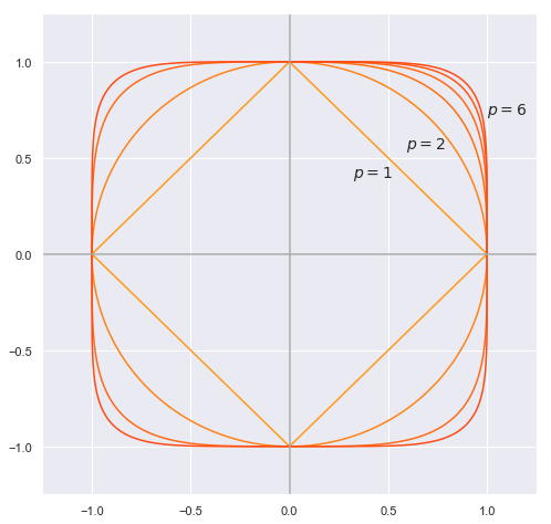

After exploring vector length I want to go back to the idea of direction of a vector. In the case of real-values vectors this can easily be described as an angle between another vector or a basis and this angle describes how “close” vectors are in space. To this end, mathematicians introduced the term dot product.

\[a \cdot b = \|a\|\|b\|cos\theta\]

where \(\|a\|\) and \(\|b\|\) are the euclidian norms and \(\theta\) is the angle between \(a\) and \(b\). In this way, the dot product is a function that takes in two vectors (of the same size) and returns a single number. But the dot product has another form which gives the same result

\[a \cdot b = a_1b_1+a_2b_2+...a_nb_n\]

The equivalence of these definitions also gives us an important inequality.

\[a \cdot b = a_1b_1+a_2b_2+...a_nb_n = \|a\|\|b\|cos\theta\le \|a\|\|b\|\]

Note that this is possible because \(cos(\theta)\le1\)

x = np.arange(-4*np.pi,4*np.pi,0.1)   # start,stop,step
y = np.sin(x)
plt.figure(figsize=(15,6))
plt.plot(x,y)
plt.plot(x,np.repeat(1,len(x)), color= '#ff9625' )
plt.plot(x,np.repeat(-1,len(x)), color= '#ff9625' )
plt.xlim(-4*np.pi, 4*np.pi)
plt.title(r'$cos(\theta)$')
plt.show()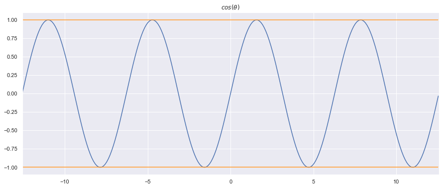

Notice also that the euclidian norm and the dot product relate as follows

\[\|a\|^2= a \cdot a = a_1^2 +a_2^2 +...+ a_n^2\]

Taking this into consideration, we square both sides of the inequality and get

\[(a_1b_1+a_2b_2+...a_nb_n)^2 \le (a_1^2 +a_2^2 +...+ a_n^2)(b_1^2 +b_2^2 +...+ b_n^2)\]

This is called the Cauchy-Schwarz inequality.

As you can see the dot product is very useful in spaces of real numbers but there are lots of vector spaces where the dot product doesn’t make sense (e.g. what is the dot product of matrices?). To resolve this, we extend to inner products of real vector spaces, which are essentially generalized dot products.

Inner products are denoted by \(\langle {a,b} \rangle\),where \(a\) and \(b\) are vectors and the output is a scalar. The important properties an inner product needs to satisfy are motivated by the dot product:

1. Distributivity: \(\langle {u + v,w} \rangle = \langle {u,w} \rangle + \langle {v,w} \rangle\)
2. Linearity: \(c\langle {v,w} \rangle = \langle {cv,w} \rangle\)
3. Commutativity: \(\langle {v,w} \rangle = \langle {w,v} \rangle\)
4. Positive-definiteness: \(\langle {v,v} \rangle > 0\) for all \(v\) and \(\langle {v,v}\rangle = 0\) if and only if \(v = 0\)

With these handy properties we can extend to more spaces(even non-numeric) and still expect the inner product to behave normally. For instance, continuous functions on an interval of \([a,b]\) form a vector space. We can define an inner product for them as

\[\langle {f,g} \rangle = \int_a^b f(x)g(x)\, dt\]

From Calculus we know that integrals have the same properties and are a valid inner product.

Even random variables, which again form a vector space, have an inner product which is defined as the joint expectation

\[\langle {X,Y} \rangle = \mathbb{E}[XY]\]